James Okamura
Rodrigo Uribe
Daniel Guzman
May 22, 2017
Introduction
In this lab, we want to apply our knowledge of moment of inertia to determine the moment of inertia or uniform triangle.
Monday, May 29, 2017
22- May - 2017 Moment of Inertia and Frictional Torque
James Okamura
Daniel Guzman
Rodrigo Uribe
May 18, 2017
May 22, 2017
Introduction
In this lab we want to know how to determine the moment of inertia of the system and determine the frictional torque.
Procedure
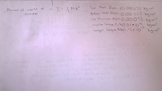
We first made measurements of various portions of our apparatus. The mass was already given to us, it was labeled on to the apparatus in grams. We measured the "thickness" or height and diameter of each cylinder using an apparatus.


Daniel Guzman
Rodrigo Uribe
May 18, 2017
May 22, 2017
Introduction
In this lab we want to know how to determine the moment of inertia of the system and determine the frictional torque.
Procedure
We first made measurements of various portions of our apparatus. The mass was already given to us, it was labeled on to the apparatus in grams. We measured the "thickness" or height and diameter of each cylinder using an apparatus.

viL

With this info, we converted the mass to kilograms and the radius and height measurements to meters and we calculated the moment of inertia of this apparatus. We were able to do this by calculating the individual parts of this apparatus, which are all rods. But before we did that, we have to determine the individual masses by taking proportion into consideration.

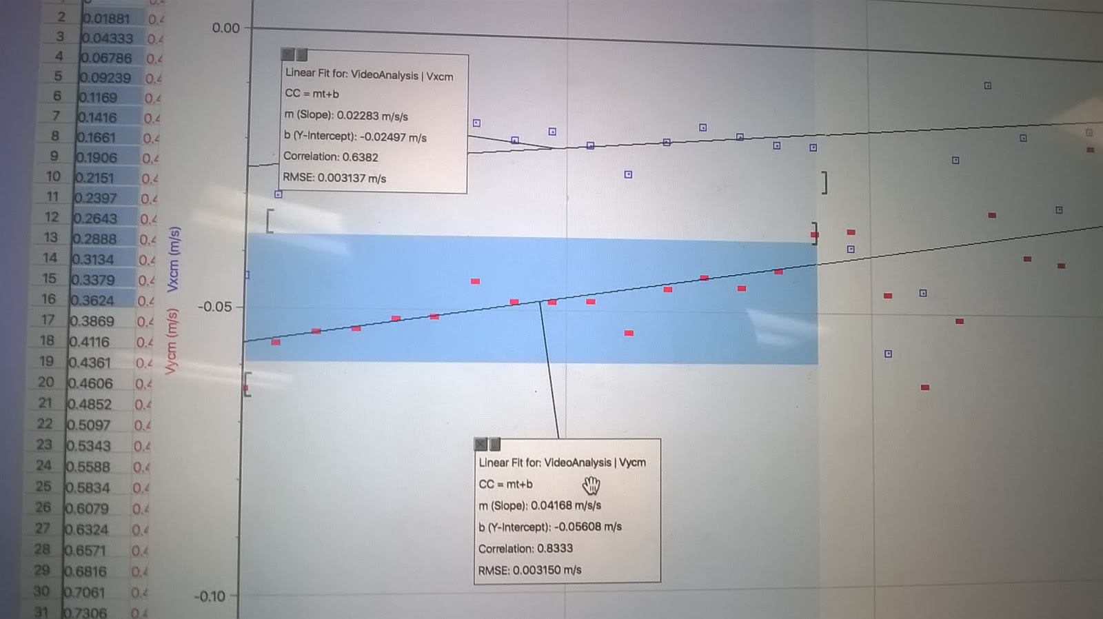
For the next part of this lab we wanted to determine the angular acceleration of the apparatus.We were able to do this by recording the apparatus in motion using a smart phone. Then we open it in Logger Pro under video analysis. We figured out the position by putting dots around the circumference. From there we were able to determine the Vx and Vy of the apparatus by taking the slope of the graphs in the x and y direction. We were able to get the magnitude of the velocity by applying Pythagorean theorem. Next if we divide that radius, we can get an omega vs. alpha graph and we took the slope of that. We were able to get the angular acceleration we needed and we were able to calculate the frictional torque.


For the last part of the lab we want to determine the time it takes for a cart to travel 1 meter, that is wrapped around the apparatus by a string. We first calculate the acceleration of the system than we were able to determine the time it too using kinematics into consideration.


Then we wanted to determine the angle of the ramp by using trignometry.
Conclusion
In this lab, I learned that we can calculate the moment o inertia of any object and with that find torque that is called by the system and the acceleration of the object.
Monday, May 22, 2017
15-May-2017 Angular Acceleration Part 1
James Okamura
Daniel Guzman
Rodrigo Uribe
May 15, 2017
Introduction
In this lab we were trying to determine what variable will affect angular acceleration, the hanging mass, the change of the spinning disk or the pulley.
Procedure:
We first made sure that all of our lab equipment was clean. From there, we made sure to take some measurements of the lab equipment as shown in the data table below. We measured the mass of each equipment using a scale and we measured the diameter using a caliper.

We first plug the power supply into the Pasco rotational sensor. If there is a cable withe the yellow paint or tape, connect only that cable to the Lab Pro at Dig/Sonic 1, so the computer is reading the top disk. If the cables are the same, connect them both. You will need to discern which is measuring the top disk and ignore the other sensor.
Set up the computer. Open the Logger Pro. There is no defined sensor for this rotational apparatus so we will need to create something that works with this equipment. Choose Rotary Motion. There are 200 marks on the top disk, so you will need to set the Equation in the Sensor Settings to 200 counts per rotation. When you collect data, you can see graphs of angular position, angular velocity and angular acceleration vs. time. the graph of angular acceleration vs. time is useless due to the poor timing resolution of the sensors. Do not use this graph.
Make sure the hose of the clamp on the bottom is open so that the bottom disk will rotate independently of the top disk when the drop pin is in place.
Turn on the compressed air so that the disks can rotate separately. You will not so much air that you op the hose from the air source, but enough to keep things smooth. Set the disks spinning freely to test the equipment.
With the string wrapped around the torque pulley and the hanging mass at its highest point, start the measurements and release the mass. Use the graphs of angular velocity to measure the angular acceleration as the mass moves down and up.

By increasing the hanging mass, we can see that the average angular mass increases. By increasing the rotating mass we can see that the angular acceleration decreases. We can see that by increasing the radius of the pulley, the angular acceleration increases.
Also in this lab we want to know the moment of inertia of the system. We can do this because we know we can calculate it by adding the various parts of each equipment inertia up.

Conclusion
In this lab I learned how various variable can affect angular acceleration in certain ways whether it be increasing or decreasing. I also learned how we can find a the moment of the system.
Wednesday, May 3, 2017
26- April - 2017 Collisions in Two Dimensions
James Okamura
Alejandro Rodriguez
April 26, 2017
In this lab, we want to see that in a two-dimensional collision and see if the momentum and energy is conserved within the collision.
We first get two balls which has relatively same mass and we put it on this glass table apparatus. On top of this apparatus is where you can put your phone to record the collision after you have changed the frame per second and to slow recording function. Also make sure the glass table is leveled, you can adjust it by changing the 3 legs of the table. Now place one of the ball on the table directly under the phone. Have your partner press record while you rolled the other ball so that it collides with the balled that was stationary and it goes in two different directions.

Now go get a laptop and open the video, edit the video so that it is the portion when the collision happens and nothing more. Now open Logger Pro and open that video file. Now you change the frame per second and starting graphing the two balls with the same masses velocities in the x-direction and the y-direction for the respective masses. Now do a linear fit to get the velocity value.


After doing this you create a new columns Xcm and Ycm and graph that . You also make graph which includes the Vxcm and Vycm.


After doing all this you want to do the same procedure again but with two different masses.


 The red and blue graphs shows the velocity in the x-direction and y-direction of the lighter mass of the two balls. The green and the brown graphs are for the bigger mass of the two balls velocity in the respective direction.
 This is the center of mass of the two balls.

Alejandro Rodriguez
April 26, 2017
In this lab, we want to see that in a two-dimensional collision and see if the momentum and energy is conserved within the collision.
We first get two balls which has relatively same mass and we put it on this glass table apparatus. On top of this apparatus is where you can put your phone to record the collision after you have changed the frame per second and to slow recording function. Also make sure the glass table is leveled, you can adjust it by changing the 3 legs of the table. Now place one of the ball on the table directly under the phone. Have your partner press record while you rolled the other ball so that it collides with the balled that was stationary and it goes in two different directions.

Now go get a laptop and open the video, edit the video so that it is the portion when the collision happens and nothing more. Now open Logger Pro and open that video file. Now you change the frame per second and starting graphing the two balls with the same masses velocities in the x-direction and the y-direction for the respective masses. Now do a linear fit to get the velocity value.


After doing this you create a new columns Xcm and Ycm and graph that . You also make graph which includes the Vxcm and Vycm.


After doing all this you want to do the same procedure again but with two different masses.

This is the collision between two different masses of balls.


This is the velocity of the balls with respective to the two balls.
Conclusion
I believe that in either part of this lab that momentum and energy is conserved. However there are some outside force as friction between the glass table and the balls that we need to take into account. In this lab I learned the concepts of momentum in two dimensions.
Wednesday, April 26, 2017
19 - April - 2017 Impulse Momentum Activity
James Okamura
Alejandro Rodriguez
April 19, 2017
Introduction
In this lab we want to see if the impulse momentum theorem can be observed. We want to test this theorem by doing one experiment in a elastic collision and inelastic collision. In the elastic collision, we do this by attaching a spring on the system and when the cart collides ( due to us providing a small force to move it) it will hit the spring and bounce back. We do the inelastic collision by having clay attached to the end of the system so when the cart collides it sticks to the clay.
We first set up the apparatus so that on one end of the track had the motion sensor and at another end of the track we set up cart with spring attach to its end so when the cart we push hits that spring it would bounce back for an elastic collision. As always we calibrate and set up the motion and force sensors. We put the force sensor on the cart. We put the cart on the track and we start the experiment. We want to see if the velocity vs time graph and the force vs time graph would produce the same results.


We first set up the apparatus so that on one end of the track had the motion sensor and at another end of the track we set up cart with spring attach to its end so when the cart we push hits that spring it would bounce back for an elastic collision. As always we calibrate and set up the motion and force sensors. We put the force sensor on the cart. We put the cart on the track and we start the experiment. We want to see if the velocity vs time graph and the force vs time graph would produce the same results.


When we try calculating impulse using the Velocity vs, Time graph and taking the integral of the Force vs, Time graph, you can see that we got two different results. I want to believe the some of the force exerted by the spring on the cart was lost when it had happen.
In this next part of this lab, we did the same thing except, instead of the spring, we had clay attached to the end so this will model an inelastic collision.


When we compare the result of our calculated impulse value compared to the integral of the Force vs. Time graph, we can see that the impulse-momentum theorem can be applied here as we got relatively similar values in this inelastic collision,
In this ab I learned that we can model both Elastic and Inelastic collision and see how the impulse-momentum theorem can be applied. That we can test this theorem using our knowledge of momentum and impulse. Although when we did our Elastic collision, our calculated value compared to the integral of the Force vs. Time graph were different.
17 - April - 2016 Magnetic Potential Energy
James Okamura
Alejandro Rodriguez
April 17, 2016
Introduction
In this lab, we wanted to test that conservation of momentum applies to this system. We have this system in which acts like an air hockey table that will act like a frictionless surface. So when we put a cart and give that cart a push, it will glide down to the edge of the system and bounce back due to the magnetic repulsion caused between the magnetic on the end of the cart and on the system.

In this lab, we first got a phone app that can measure degrees the system is raised from the horizontal, and place it flat from the horizontal.
Next, we raise the system some degrees, turn on the system and gently push the glider so that is slides down the ramp and get push back by the end of the magnetic repulsion and let the cart glider comes to an equilibrium distance. We record the degrees of how much the system was raised and the distance the cart glider has traveled back due to the magnetic repulsion. We repeat this process at least another 4 times and record the distance from the end of system and degrees. We then convert the angle from degrees to radians and then use that to calculate the force.


In this next part of the lab, we attached an aluminum reflector on top of the cart and weighed the whole cart.
Next we placed the cart relatively close to the end of the ramp and turned on the air. We ran a motion detector. We then determine the relationship between the distance the motion sensor reads the distance we measure between the two magnets,
We then set the motion to record 30 measurement per second. Then we created a new column for this separation by magnets measured by the motion detector.
We then start with the cart at the other end of the cart, start the detector and push the cart with a gentle push.
We then made a graph that had the work done by the magnets and the kinetic energy.

The above graph shows the energy caused by the magnets and the kinetic energy. When you add the energy of both these graphs, you can see the total energy, the energy conserved by the system.
In this lab, I learned that energy is conserved by the system. That whatever energy you start out with is what you should end with unless there's an external force ( in this case there was none). I learned how we can calculated the work done by the magnets by using a free body diagram.
Monday, April 17, 2017
10 - April - 2017 Work- Kinetic Energy Theorem Activity
James Okamura
Jin Im
April 10, 2017
Introduction
In this lab, we are trying to explore the relationship between work done by and kinetic energy of an object. We can do this by having a cart on platform with a string attached to it with a hanging mass to the other end of the string.
We first gt a track and we put our cart with the force sensor on it. Then on one end of the cart we attach a string to it and on the other end of the string we attach 50 grams of hanging mass. On the other end of the track we put a motion sensor on it. We calibrate the force sensor.

Next we open the document as posted in the lab manual and we put the cart as shown in the diagram and click record, and let the experiment began. We get a graph like this .

We get this graph after we selected the Force vs, Time graph, changing the x-axis and y-axis and then taking the integral of the graph. our integral value we get is 0.1842 while our kinetic energy value is 0.186 J. This is true because the only work the cart is doing is kinetic energy when the cart goes at some velocity after the cart is let go causing the hanging mass to pull the cart forth.
In this next part of the lab, we want to attack a spring to the end of the force sensor and stretch and let it go after we stretch the spring a certain distance.
The set up is the same except for the opposite end of the motion sensor that is where we attach one end of the spring and the other end to the cart. We then stretch the cart a certain distance and let it go. In this lab, not only do we have work done by kinetic energy but also with the elastic potential energy.


The above graph is the integral of the kinetic energy graph and the other one is the graph cause by elastic potential energy.

This is the graph we have watched where a professor pulled a rubber band back. When you see integration of this graph and the work done by Kinetic Energy, they are quite similar.
In this graph I learned that we can learn and use what we know of the Kinetic Energy Theorem. We have seen this application when doing this lab.
Wednesday, April 12, 2017
5 - April - 2017 Work and Power
James Okamura
Alejandro Rodrigues
Rodrigo Uribe
Daniel Guzman
April 5. 2017
Introduction
In this lab, we were trying to determine how much energy ( in joules ) we use in our daily activities such as lifting, running and walking that we do everyday. This is important to know as we use up a lot of energy in the daily activities we partake each day and we want to determine how we use up the energy in our bodies.
In this lab, we set up this pulley-like system at the to of balcony on the second floor of Building 60 outside. With this we run a rope through it and have one end of rope attached to a backpack that has some weight to it and we lift it. We also record the time it took for us to lift the backpack from the the ground level to the edge of the balcony.
In the next part of the lab, we timed ourselves where we would walk and run up the steps from the ground level to the second floor. We also measured how high each step is with a meter stick and counted how many steps there are. By multiplying those two values and applying trigonometry to it we can determine the distance we travel.


Procedure
We first set up the pulley on a board and have one person put their feet on this board. Next we put a rope through the pulley. We attach one end of the rope to a backpack which have some weights inside ( for our experiment, we put in 9 Kg) . Next, we get ready by putting gloves on ( to prevent rope burn ) and holding on to the other end of the rope. We start pulling the rope to the height we want to pull to, which this case was the edge of the balcony of building 60. While someone is pulling the backpack to its desired height, your partner is measure the time it takes (in seconds ) with a stopwatch.
We later on walk up the stairs ( which we measure the height of a step and multiply by the number of steps). We timed how long it took to climb the steps.
After that, we later run up the steps. Time how long it took.
We calculate the power output for lifting, walking and running respectively.


Conclusion


I learn in this lab is that, I can apply the knowledge i have in calculating work and power to determine how much work and power I do when doing everyday things such as lifting something heavy or covering long distances by walking or running.
5- April - 2017 Centripedal force with a motor
James Okamura
Daniel Guzman
Rodrigo Uribe
Alejandro Rodriquez
April 5, 2017
Introduction
In this Lab, we are trying to figure out the relationship between theta and omega.
In this lab, we start with this apparatus that looks like a tripod and has a motor on the top. Connected to the motor has some rod. At one end of this is a string attached to it. The other end of the string has a mass to it. Put a piece of tape to the block. From a certain distance you set up a ring stand with photo gate on it , and you adjust it so the tape will pass through the photo gate. From this you can determine the time it takes to have one full revolution.


We can get the angle from looking at the right triangle with hypotenuse L and height H-h.
We can get the rotational speed by collecting how long it take to have ten rotations and divide that by ten.
We measure the height of the apparatus and how high off the ground the hanging mass is.
With this given info, we can calculate the rotational speed by applying free body diagram and by using the the period of 10 rotations.
After collecting data after 5 trials, we can calculate its respective rotational speed.
We can now compare the model and rotational by putting it on a graph and getting a linear fit.
We can then calculate the percent error by using the the slope of our graph as the experimental and the actual value of rotational speed as 1 radians/ second.


Conclusion
In this lab, I learned that we can apply our knowledge of Centripedal Force to real life application. I learned that although there is not that much difference from our model and actual omega, I think I would calculate omega by using the period of rotation since I would not get too much of an error.
Subscribe to:
Comments (Atom)